Analog to Digital Converter (ADC)
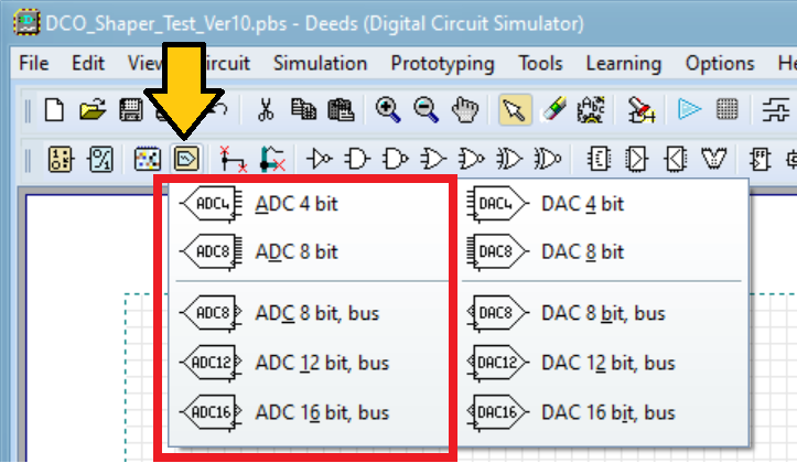
The component bar offers Analog-to-Digital Converter (ADC) components in a range of bit sizes, including 4, 8, 12, and 16 bits (see the following figure).
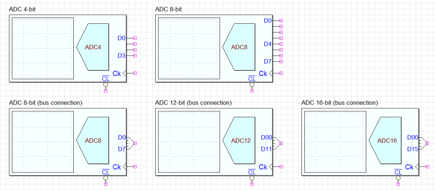
Symbols for ADCs in schematics are depicted by an empty square to the left and a pentagon to the right, representing the converter's functionality (see below).
Analog signals are virtually acquired by ADC components, converted to digital, and then transmitted to the connected digital network for processing.
The ADC components within the Deeds simulation environment do not acquire signals from the real world. Instead, the virtual signal sources available for the ADC are the Analog Generator, or a Samples File.
- Analog Generator:
The ADC can sample common laboratory waveforms such as sine, triangle, square, Fourier synthesized signals, and white noise using a versatile built-in analog signal generator. - Samples File:
The ADC can generate a sequence of digitized samples from a CSV (Comma Separated Values) file to simulate the sampling of any analog signal.
The signal waveform, regardless of its source, is drawn within the square area of the ADC symbol during the simulation. This is achieved by digitally converting the signal values and plotting them 'by a pen,' resulting in a chart that resembles the output of DAC components (see the screenshot below).
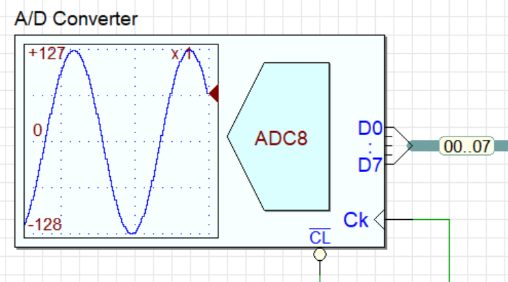
The ADC functions as a parallel register on the output side, producing a new value that is also added to the display chart with each positive edge of the clock (Ck). The output register is cleared, and data conversion is halted, when the clear input (!CL) is activated.
Inserting an ADC component in the circuit
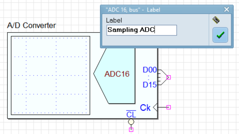
A dialog box will appear after the ADC component is placed and inserted into the circuit, prompting the user to assign a name to the ADC (see the example below).
The connection of the reset network and the clock should be defined before defining the properties of the signal source for the ADC (see the example below).
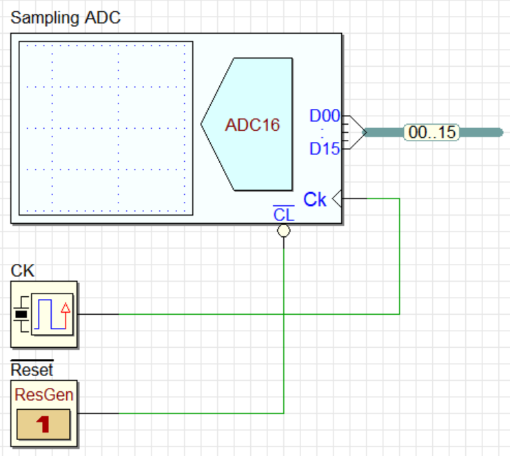
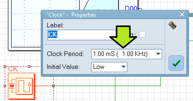
The ADC component can automatically determine the sampling rate from the clock generator settings when a clock generator is directly connected to the ADC's clock input using a wire. This is the easiest way to assign the sampling rate, although it can also be done manually. In this instance, the clock frequency is set to 1.0 KHz.
ADC simulated signal sources
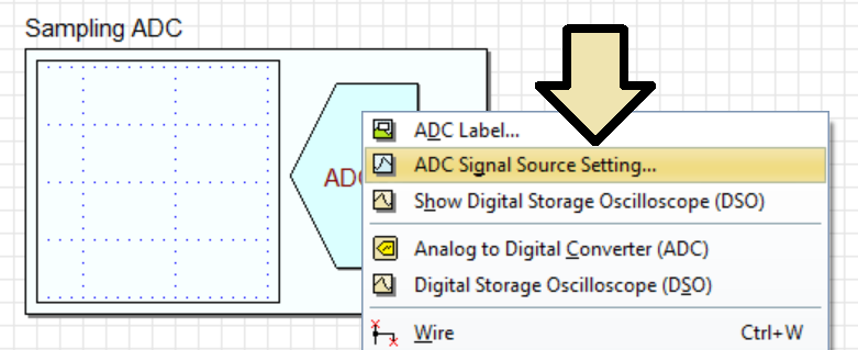
To adjust the properties of the simulated signal source for the ADC, double-click on the component, or access the command from the context menu, as shown below.
The following dialog will be displayed alongside the component.
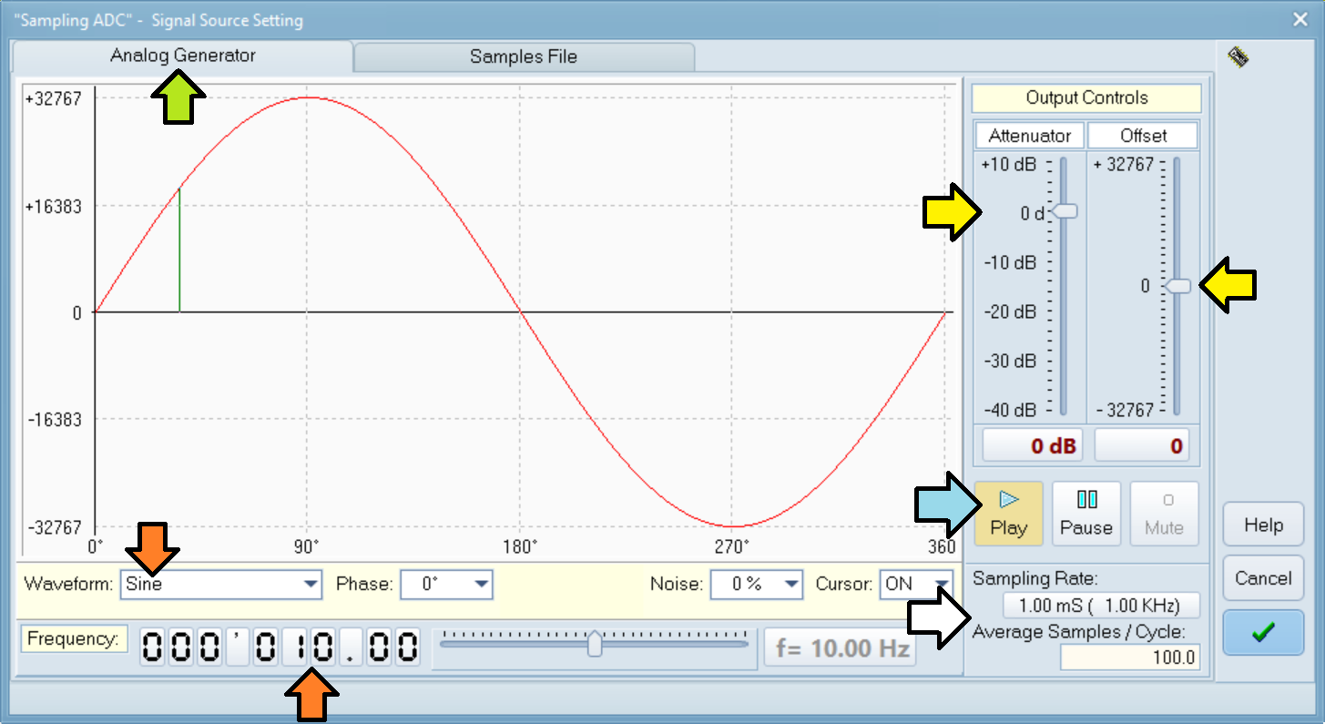
The default settings are displayed. Let's focus on the key elements highlighted in the screenshot.
- The Analog Generator page is chosen by default, which is indicated by a green arrow.
- The waveform to be generated is defined as sinusoidal, with a frequency of 10 Hz (orange arrows).
- The sampled sine wave values will range from +32767 to -32767. This is due to the 16-bit ADC and the output controls on the right, which are set to zero vertical offset and no attenuation (0 dB) (yellow arrows).
- The clock connected has a frequency of 1.0 KHz, which determines the sampling rate. This configuration results in 100 samples per cycle (white arrow), calculated as 1000 samples per second divided by 10 cycles per second.
- The animated simulation will start with signal generation active immediately because the Play and Pause buttons are set to Play (turquoise arrow).
To finalize our schematic, click the OK button to accept the default settings. Next, incorporate a DAC component to replicate the ADC output. Lastly, activate the clock animation (red arrow) and adjust it to a frequency of 50 Hz (green arrows), as shown below (click on the figure to open the circuit in Deeds-DcS).

The animated simulation is demonstrated in the following video, which can be downloaded in full resolution here.
The initial click on the DAC opens the window of the corresponding DSO. Subsequently, clicking on the ADC opens both its DSO and the control window of the associated generator. This window, which closely resembles the configuration dialog mentioned earlier, allows for real-time control of the generated signal's parameters. This functionality is demonstrated in the video, where the frequency slider is dragged with the mouse to dynamically increase and decrease the frequency.
Now, close the simulation and double-click the component symbol to reopen the ADC configuration dialog. Then, select the Samples File page (see the green arrow in the screenshot below).
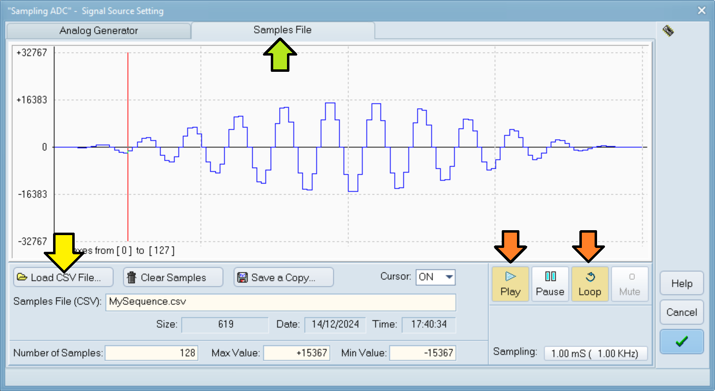
The diagram is typically empty by default. However, in this instance, we have already utilized the button indicated by the yellow arrow to import a CSV File containing samples of an arbitrary waveform.
The samples are displayed in the graph. The file MySequence.csv contains 128 samples, with values ranging between +15367 and -15367, as shown. The active Play and Loop buttons indicate that the sequence, once the simulation begins, will play immediately and continuously loop (see the red arrows).
A downloadable copy of MySequence.csv, viewable in any text editor, is available here.
Let's restart the simulation. The following video provides an example of an animated simulation. For full resolution, download the video here.
We observe the following from the video:
- The animated simulation starts at the beginning of the video.
- The DSO and Generator windows open automatically (they were set to open when the simulation started).
- After the timed reset, the sample sequence immediately starts to be generated (cyclically, as expected).
- The Loop button is deactivated by the user's click during the sequence's third iteration.
- The DSOs indicate that the sequence terminates and does not recur (the generator has been paused).
- The user pressed Play, and the sample sequence started again. Notice that the sequence does not repeat, because Loop mode had been deactivated.
- The user then demonstrates that it is possible to switch between the Analog Generator and Sample File generation modes during execution.
A complete description of the generator's features and settings
can be found here.
Information on using the DSO is
available here.
ADC Simulation in the Timing Diagram Window
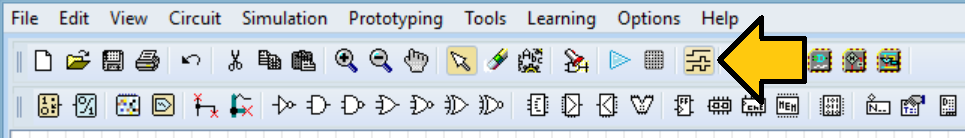
The schematic shows a demonstration circuit where signals from two ADCs are multiplied together using an 8x8 bit digital multiplier (indicated by the arrow). The "Carrier" ADC (top left) is programmed to capture a 2KHz sine wave, while the "Modulation" ADC digitalizes a 100Hz sine wave. The output is displayed by a DAC.

Access the Timing Simulation Window through the highlighted command (see image below).
The image below displays the Timing Simulation Window, which shows a test sequence (automatically loaded on opening because previously defined by the user as default).
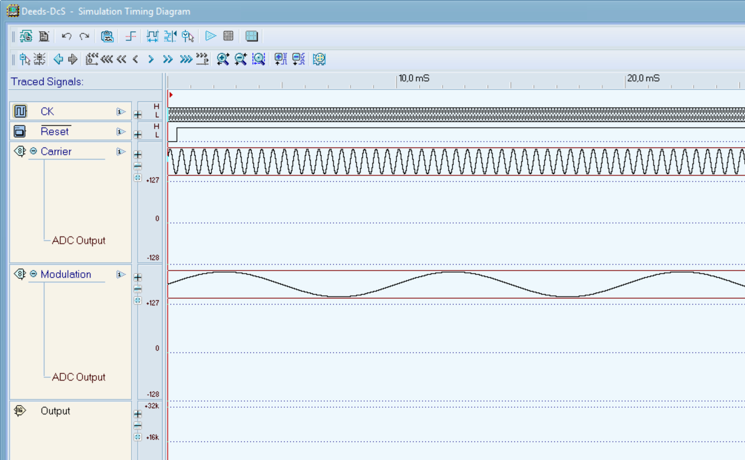
The clock and reset traces are followed by those of the two ADCs. The DAC trace is partially displayed at the bottom. The ADCs currently only display the waveforms set in the respective generators (in the main trace), as the simulation has not yet started. All the ADC and DAC output traces appear still blank.
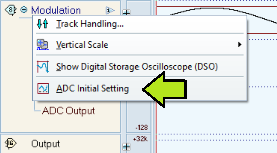
The initial settings of the trace were copied from the ADC generator settings assigned in the schematic, unchanged. These settings can be modified by clicking on the track name, which will display a context menu (see below). Select "ADC Initial Setting" from the context menu to change the initial setting.
The previously seen content appears in a dialog box, as shown below.
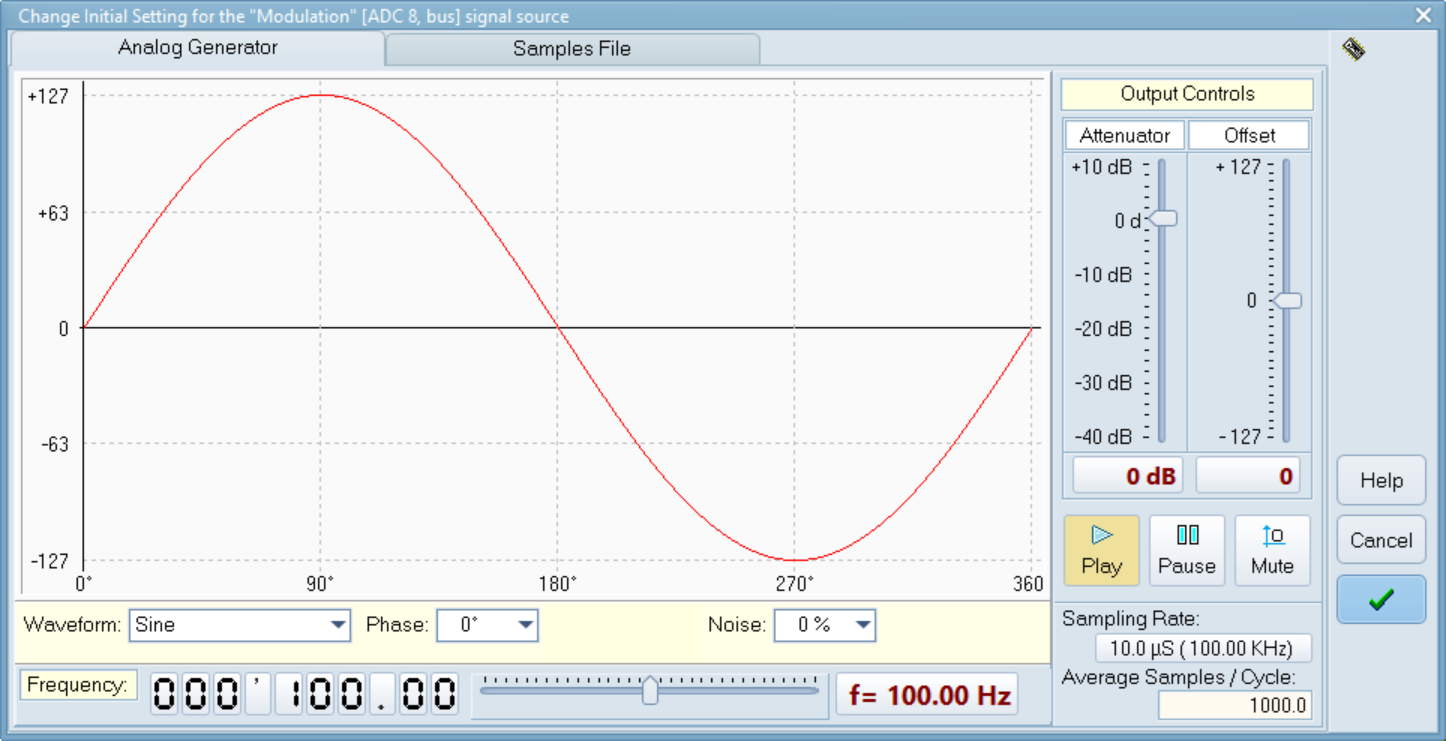
In this case, we can disregard modifying the initial values and proceed with the simulation. The subsequent screen will be displayed.
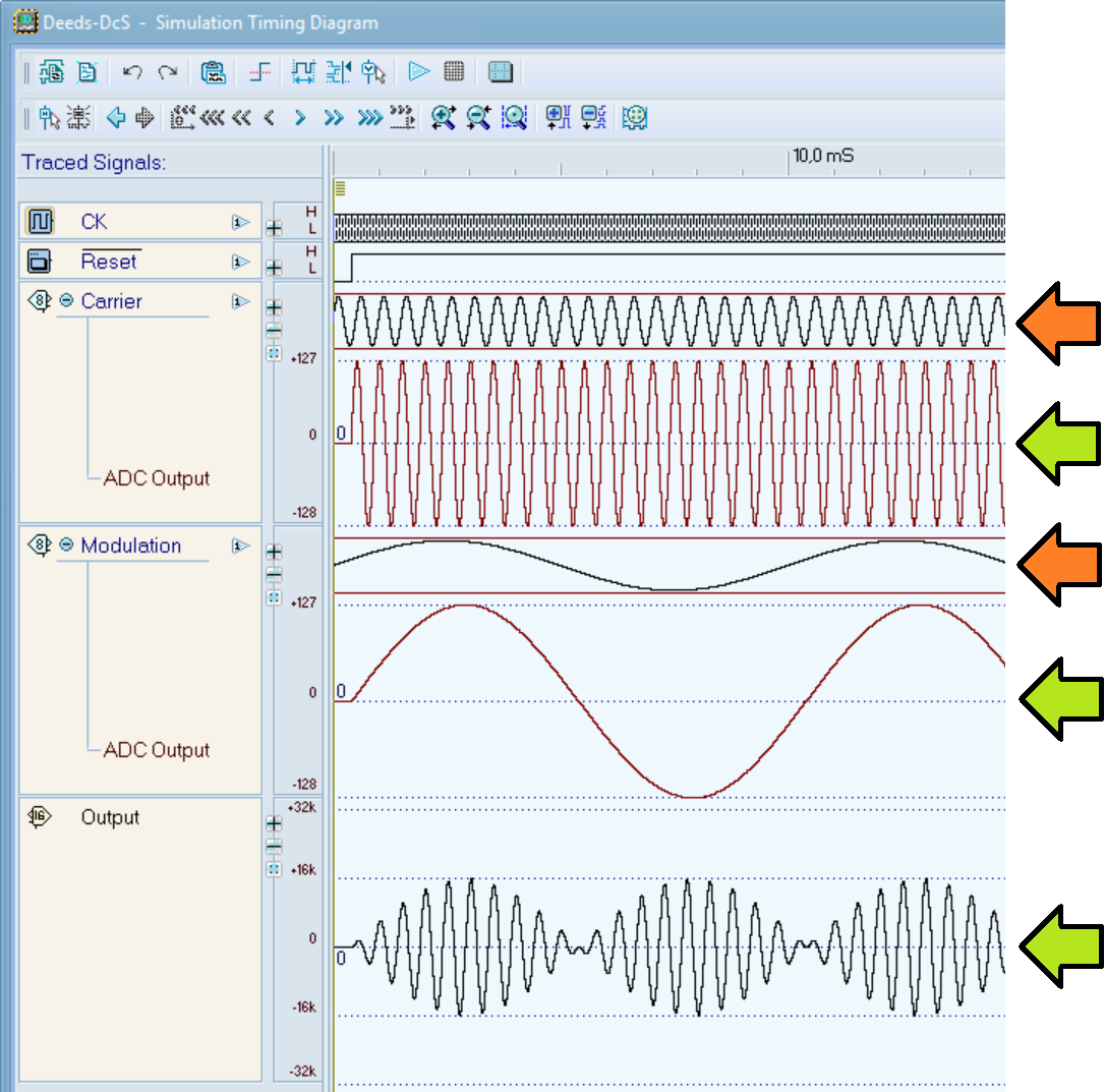
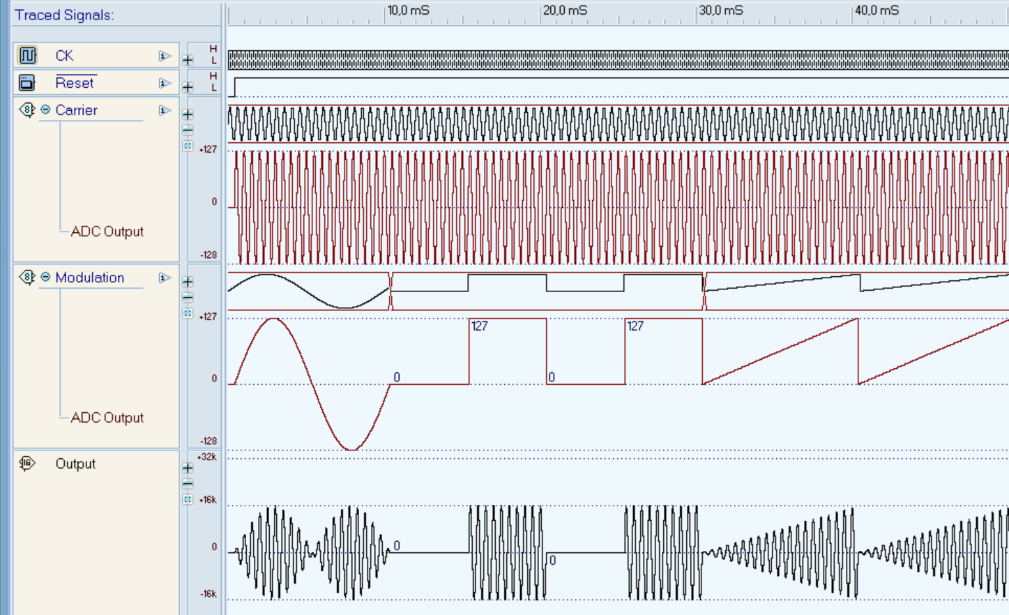
The green arrows in the figure above show the timing simulation results for both the ADC outputs and the DAC output. The traces indicated by the red arrows are not results, but reminders of the generator settings. For clarity, see the zoomed-in timing diagram view below.
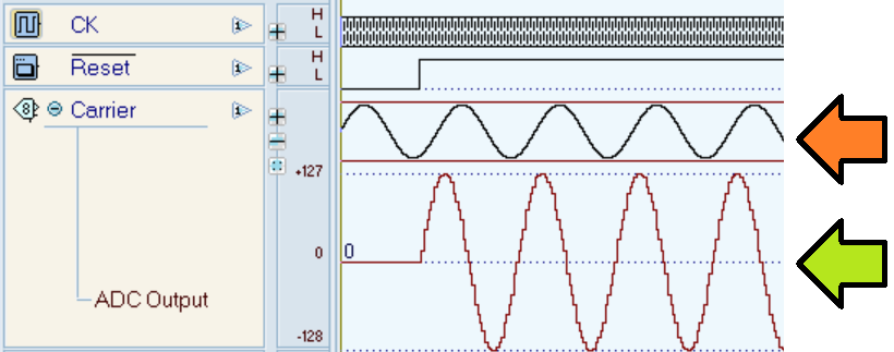
The sinusoid generated by the ADC begins at the moment the reset signal is deactivated, as expected (green arrow). In contrast, the trace indicated by the red arrow is unaffected by the reset signal, as it serves only as a reminder of the generator settings.
The ADC main trace can be clicked on to adjust the generator settings over time. The modulation waveform could be changed around 10mS, for instance. To enable the new setting insertion command, click on the relevant track (shown below).
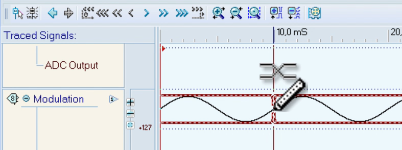
The dialog box, which allows you to define a new generator setting (as shown in the screenshot below), will open when you click again to choose the time of the change.
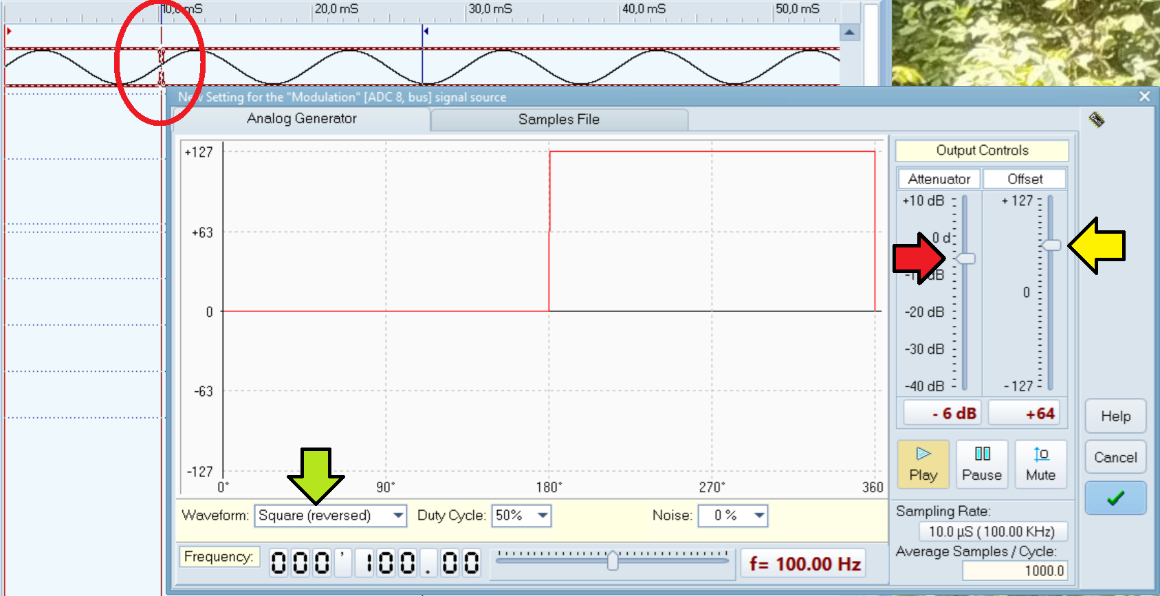
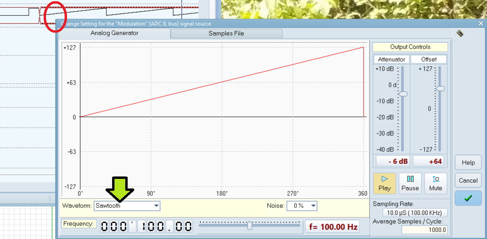
The time of the mouse click is highlighted by the red ellipse. We select the following:
- The reversed square waveform (green arrow);
- An attenuation of -6 dB (red arrow);
- An offset of +64 (yellow arrow).
The resulting signal will be zero during the first half of the cycle and reach its maximum positive value in the second half. As the simulation will demonstrate, the output signal from the multiplier will result in a burst, at zero amplitude for half the time and maximum amplitude for the remaining half.
Other setting variations can be defined in time using a similar procedure. A suitable test sequence, accessible via the command shown in the figure below, has already been prepared with two setting changes.
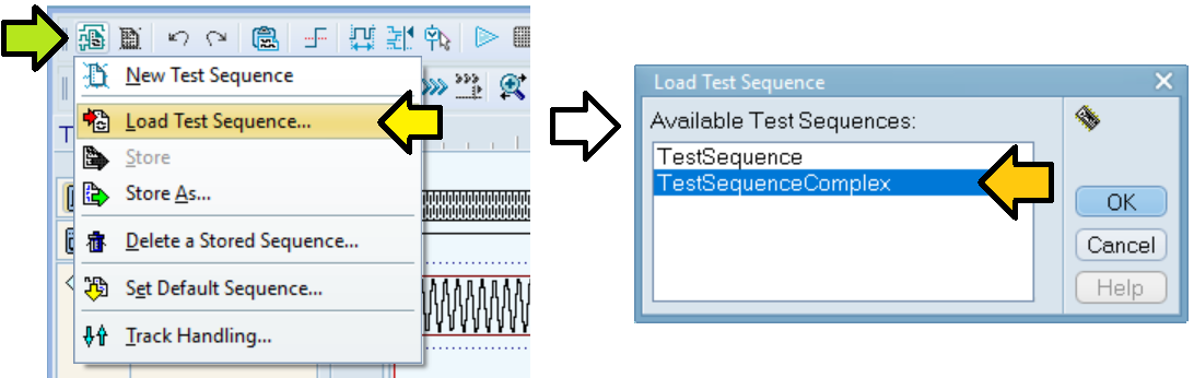
The results shown below were obtained after running the simulation.
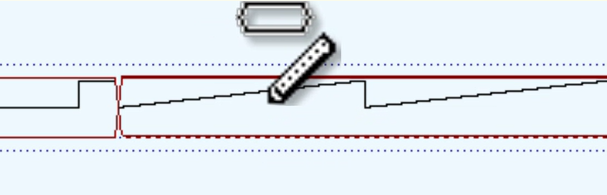
To move a generator setting transition, simply hover your mouse over the transition and click to drag it to a new time.
![]()
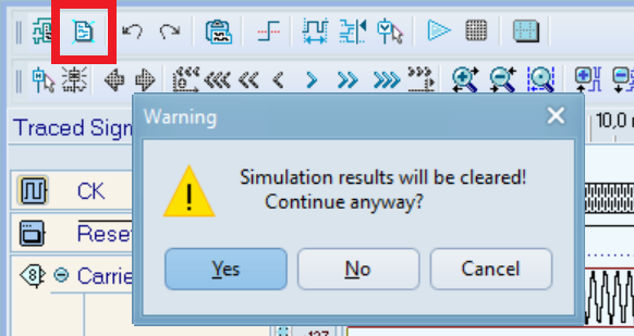
To change a test sequence, either select a time following the end of the previous simulation or use the highlighted command to remove all the simulation results (see below).
To examine (or modify) the generator settings of a particular section, hold down the CTRL key and click on the desired section. Let's illustrate this with the third section of the "Modulation" ADC main trace; we'll check its configuration without making any modifications.
The waveform was changed to "Sawtooth", but the -6dB attenuation and +64 offset were kept (see below). This is the only change from the previous section.