Digital Storage Oscilloscope (DSO)

The Digital Storage Oscilloscope (DSO) is a tool associated with the DAC (Digital to Analog Converter) and ADC (Analog to Digital Converter) components in Deeds simulation software. It replicates the main feature of a real digital oscilloscope, providing a visual representation of digital signals waveform. Note that the DSO is not a component itself.

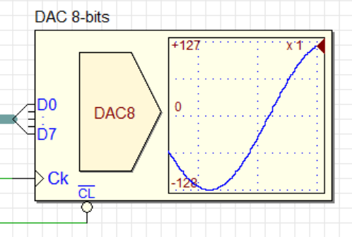
The DAC and ADC component symbols have a small square display. During simulation, the virtual representation of the signal that a real DAC or ADC would produce is displayed directly on the component symbol (see the 8-bit DAC example shown below).

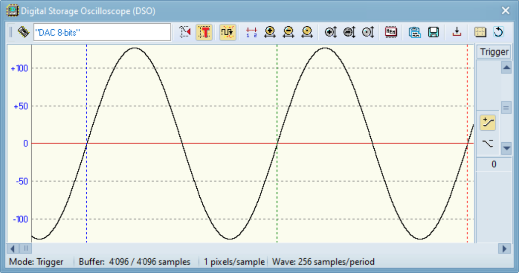
However, this method of displaying the signal has considerable limitations and is only adequate for rudimentary applications. To address these constraints, Deeds offers a unique tool that emulates the primary function of a physical instrument: the Digital Storage Oscilloscope (DSO). Refer to the screenshot below for an example of the DSO window.

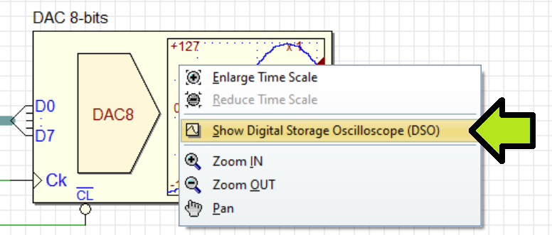
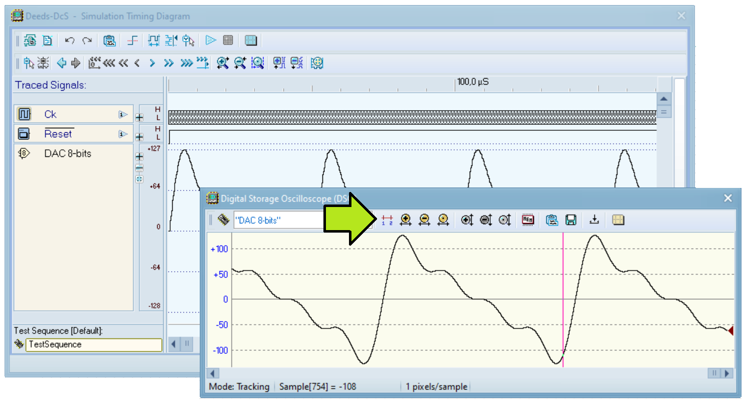
When simulating a circuit, clicking on a DAC or ADC component will launch the DSO window. Alternatively, you can right-click on the component and select it from the context menu (as shown in the image below).

Upon opening the window, users have the flexibility to position and resize it according to their preferences. Notably, upon subsequent reopenings, the window will automatically retain its previous position and dimensions, ensuring a consistent and personalized user experience.

DSO Key Features

1. Tracking and Trigger Mode:
   The DSO can operate in either Tracking Mode or Trigger Mode. In Tracking Mode, the oscilloscope is in continuous acquisition mode, with automatic scrolling to the left of the already acquired samples. In Trigger Mode, the display can be frozen in a fixed position, definable by adjusting the level of the trigger threshold and the relative slope.
2. Horizontal and Vertical Zoom:
   The DSO allows for horizontal and vertical zooming of the waveform drawing, enabling users to focus on specific details of the signal.
3. Memory Buffer Size:
   The size of the sample memory buffer can be adjusted from 256 to 1M samples, allowing for the capture of different lengths of waveforms.
4. Data Export:
   The DSO provides options to save the current view of the waveform drawing as an image to the clipboard and export the samples present in the buffer to a comma-separated values (CSV) text file.
5. Settings Persistence:
   The DSO settings can be made persistent by saving them in the circuit file, allowing users to easily access the same settings when reopening the circuit.
6. Automatic DSO Re-opening:
   The DSO window can be set to automatically reopen when the simulation starts, providing convenient access to waveform visualization.

DSO Commands

Tool Bar

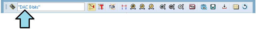
The following figure presents the command toolbar. The arrow indicates the field that displays the label previously assigned to the corresponding component.

Tracking and Trigger Modes

The adjacent illustration showcases two buttons that enable the user to effortlessly switch between the two operating modes of the oscilloscope. Pressing the left one sets the Tracking Mode, while pressing the other one sets the Trigger Mode (the two modes are mutually exclusive).

In Tracking Mode, the oscilloscope functions in persistent acquisition mode, the default setting. In this mode, samples are continuously acquired and automatically scrolled to the left on the display. This automatic scrolling is indicated by the green arrow in the adjacent figure.

In this mode, the drawing's right edge aligns with the window's edge by default. Nevertheless, you can move the view using the horizontal scroll bar at the window's bottom. The waveform drawing emphasizes the latest sample acquired, which is the one furthest to the right (represented by the yellow arrow in the figure above). Essentially, the 'pen' will seem to trace the line, sample by sample, as it does in the component symbol.

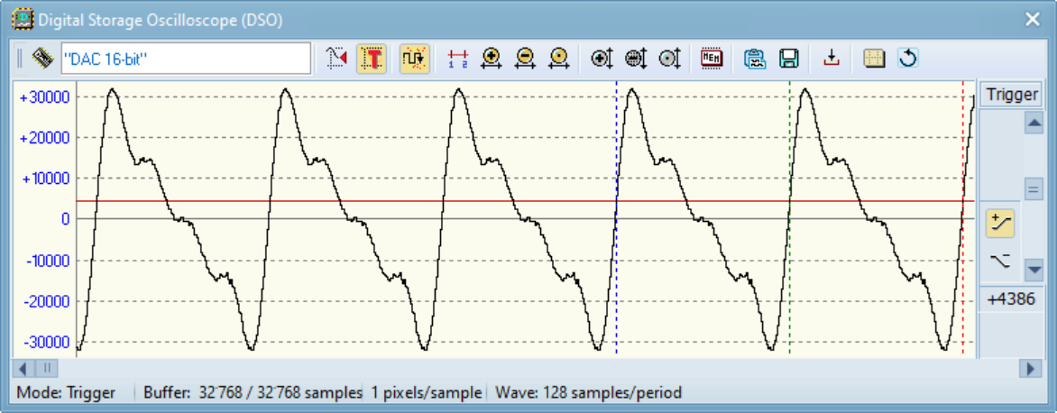
In Trigger Mode the oscilloscope behaves exactly as expected in a real instrument. In this operating mode, the display can be frozen (synchronized) in a fixed position. This position is definable by adjusting the level of the trigger threshold and the relative slope. A vertical panel is displayed on the right side of the window. This is illustrated in the next figure.

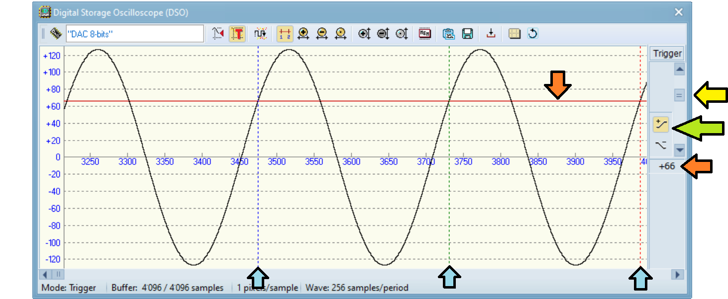
The vertical scroll bar (yellow arrow) permits to define the trigger threshold level, while two buttons [+] and [-] (green arrow) set the requested signal slope in the trigger point. The value of the chosen trigger threshold is also displayed (red arrows) as a number and as a horizontal line in the drawing.

During the wait for a trigger threshold with a desired slope, the waveform is displayed flowing to the left, similar to Tracking Mode. Once the trigger is detected, the waveform stops moving, and a vertical dashed line is drawn at the point where it crossed the threshold. Up to three such trigger instants are displayed, as indicated by the blue arrows in the figure above.

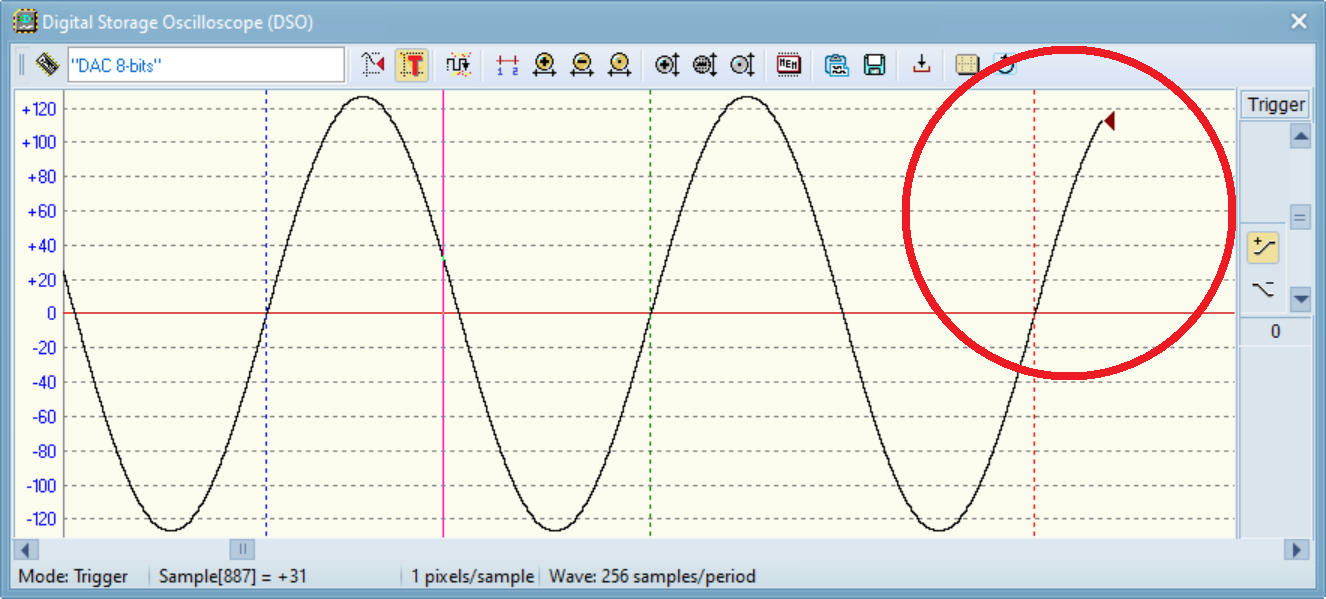
By utilizing the horizontal scroll bar (as depicted in the following figure) and shifting the view slightly to the right, we can observe the sequential arrival of new samples. Meanwhile, the remainder of the waveform drawing stays fixed on the trigger points, allowing for continuous monitoring of the signal.

Clock Animation

In the image provided, the clock animation toggle button is prominently featured.

From an educational perspective, the simulation clock animation can be paused to enable a thorough examination of the circuit's behavior and waveforms. This feature, accessible at the bottom of the main window, offers the same functionality as the main window's clock animation.

Horizontal Axis

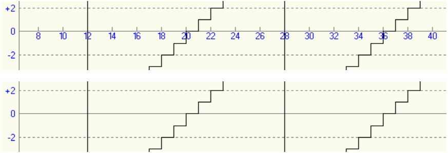
In the image below, the highlighted toggle button lets you show or hide the horizontal scale. This scale enumerates the samples in the memory buffer.

Here is the same detailed waveform drawing, presented with and without the numbered scale for comparison.

Horizontal Zoom In/Out

In the provided figure, the three highlighted buttons control the horizontal zoom of the drawing. The (+) button is used to zoom in, the (-) button is used to zoom out, and the third button enables you to view the entire acquisition. The zoom range varies from 256 pixels per sample to 2048 samples per pixel.

Vertical Zoom In/Out

The vertical zoom of the drawing is controlled by three buttons, as illustrated in the following figure. The (+) button zooms in, the (-) button zooms out, and the third button adjusts the vertical zoom to match the maximum amplitude of the digital signal.

Vertical Axis

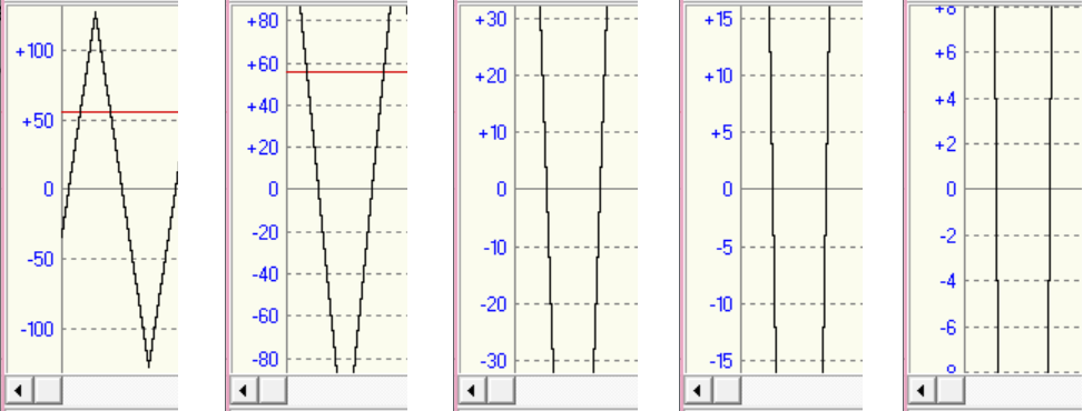
On the left side of the drawing, the numerical scale of the vertical axis is consistently displayed. The density of the scale adjusts automatically based on the current vertical magnification. Several examples of this can be seen in the following figure.

Memory Buffer Size

In the figure provided, the highlighted button enables you to specify the sample memory buffer's size. By default, it's set to 4K, but you can modify it to range from 256 to 1 million samples.

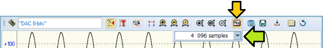
The buffer size is adjustable, even when the animation clock is active. However, if the requested size is smaller than the current buffer, the user will be notified that the oldest samples exceeding the new buffer size will be discarded.

Hardcopy Current View on Clipboard

To preserve the current appearance of the waveform drawing, you can save it as an image to the clipboard. The button for this action is illustrated in the figure below.

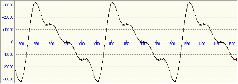
In the following figure, you will see an example of an image that has been saved to the clipboard. Please note that the only part included is the diagram area.

Saving Data as Comma Separated Value (CSV) file

In the adjacent image, you can see a button marked by a red frame. This button allows you to save the samples currently present in the buffer as a comma-separated values (CSV) text file.

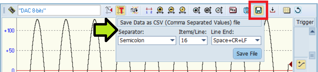
The button presented in the figure opens a panel containing controls used to specify the desired file format. The data can be separated by different combinations of Comma, Semicolon, Space, and Tab characters. Each line can accommodate 1, 4, 8, 16, 32, or 64 numbers and can be concluded by various combinations of Space, Carriage Return and Line Feed characters. The file is saved with the '.csv' extension, and the format illustrated in the figure has been proven readable by the majority of commonly used spreadsheet applications.

Saving Oscilloscope Setup

Using the button highlighted in the adjacent figure, you can make the oscilloscope settings permanent. This enables you to store them in the circuit file, ensuring that any adjustments to the parameters are retained. Without this feature, any changes made would be temporary and would not persist once the oscilloscope is turned off or the circuit file is closed.

Upon pressing this button, a warning message will appear, informing the user that the current configuration will be saved to the circuit file (in the context of the associated DAC or ADC component):

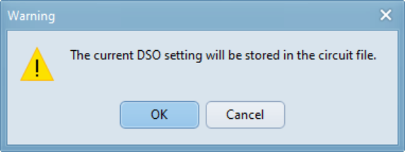
After exiting the simulation, please remember to save the file from the main window, as it will be modified. The settings will be saved individually for each DAC (or ADC) component in the circuit. It's important to note that saving the parameters will create an UNDO entry, allowing you to revert the operation if needed.

Drawing colors setting

In the next figure, the arrow points to the penultimate button on the toolbar. By clicking this button, a menu with four options appears, providing a choice between four different color sets to depict the waveform.

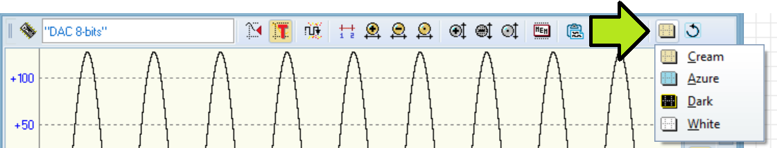
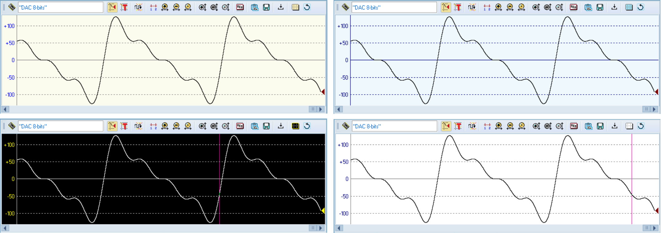
In sequential order, the following figure illustrates four options: 'Cream', 'Azure', 'Dark' and 'White'.

Automatic DSO re-opening

To the right of the toolbar (as shown in the figure below), there is a button that allows users to set the DSO window to automatically reopen when the simulation begins.

Within the system Registry, not only is the position of the DSO window stored but also its dimensions, alongside other crucial information.

Status Bar

Located at the bottom of the window, the Status Bar is highlighted in the figure below.

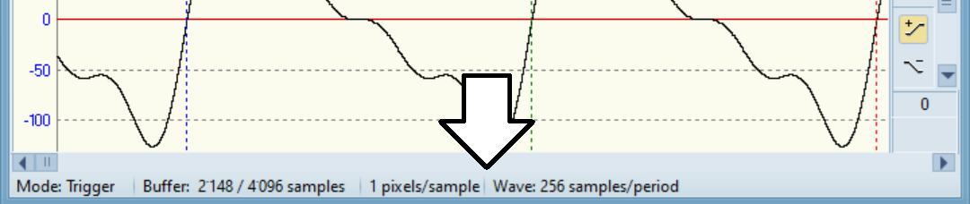
The Status Bar is divided into four fields:

• The first field on the left indicates the current mode, either Tracking or Trigger Mode".
• The second field, if the clock animation is active, displays the number of samples acquired as a function of the buffer size. If the animation is inactive, this field shows the index and value of the sample pointed to by the mouse cursor.
• The third field shows the horizontal scale of the waveform in terms of pixels per sample or samples per pixel, depending on the zoom level.
• The last field is only active in Trigger mode and displays the waveform period, calculated as the number of samples that occurred between the last and previous trigger instances.

In the following example, the animation clock has been stopped using the stop button (indicated by the green arrow).

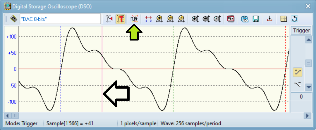
The white arrow shows a vertical cursor that follows the mouse movement. According to the second field of the status bar, we see that sample at that cursor position is located at index 1566 of the memory buffer, and its value is +41.

The oscilloscope and the Timing Diagram.

In the Timing Diagram simulation mode, you can display the oscilloscope window. It's important to note that the waveform drawing is only updated at the conclusion of each simulation interval.

When the Timing Diagram Window is active, the oscilloscope can be opened by clicking on the DAC component. Alternatively, a helpful menu item in the DAC track allows you to show or hide the corresponding oscilloscope (refer to the next figure).

In the Timing Simulation, the automatic window reopening option is disabled, making the button invisible in the DSO toolbar. Additionally, the clock animation and mode selection buttons, which are always set to Tracking in this mode, are hidden from view. Refer to the following figure for a visual representation of this.

A working example

The following diagram illustrates a test circuit that allows you to explore the capabilities of the oscilloscope. By clicking on the figure, you can access the circuit in the Deeds-DcS in Auto-Play Mode, enabling you to interact with and manipulate the oscilloscope's functionalities. This circuit is a programmable frequency signal generator that generates a signal whose frequency is directly proportional to the FREQ parameter.

The computing network on the left adds the FREQ parameter to the contents of the parallel register at each rising edge of the clock. The register addresses the ROM, which stores samples of a complete cycle of the waveform. The DAC then outputs the generated signal.

When you open the file, the simulation will automatically start due to the enabled Auto-Play Mode. To view the generated waveform, simply click on the DAC component. The oscilloscope will open, displaying the waveform. By changing the FREQ setting, you can change the frequency of the generated waveform and observe the changes in the time graph produced by the DSO.

Here's a brief video showcasing the network simulation and the visual representation of waveforms on an oscilloscope:

You can download the video in full resolution here.