 Deeds-DcS Timing Diagram Simulation
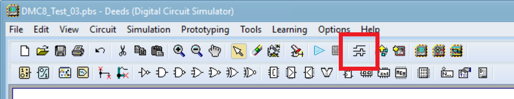
In the toolbar of the Deeds-DcS main window we find the command to access the Timing Simulation window (highlighted in the following screenshot).
...To be completed... 
Index
Signal Editing
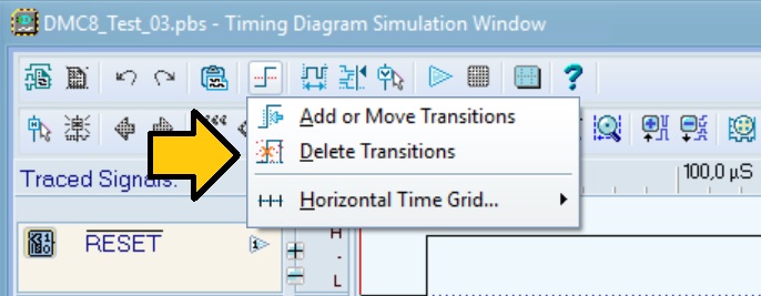
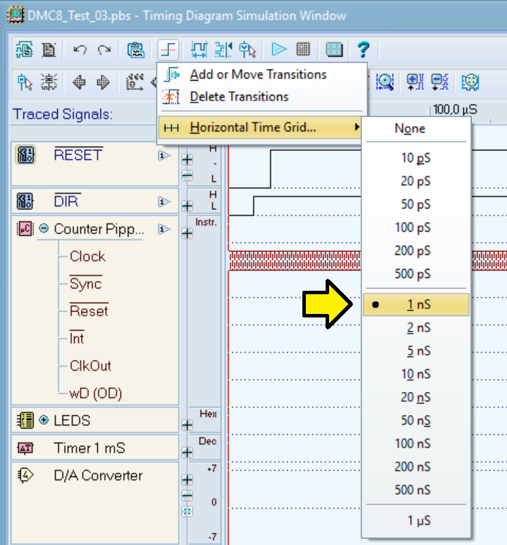
The upper toolbar in the Timing Diagram window offers a single icon to open the signal editing command. It brings up a menu with the commands 'Add or Move Transitions', 'Delete Transitions' and 'Horizontal Time Grid' item (see below).
Adding or Moving Transitions
...To be completed...
Adding a Pulse Train You can add a pulse train to a single-wire input using the 'Add Pulse Train' command, found in the trace button drop-down menu (see the example below).
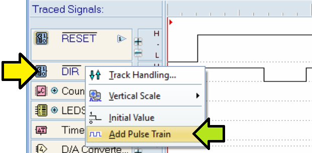
The signal trace may already contain transitions. The pulse train will be added after these transitions, if they are present, otherwise the pulse train will start from time zero. Clicking on the command will open the dialog box shown below.
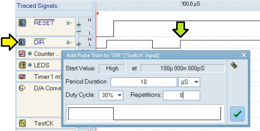
At the top of the dialog area we see a Start Value = High (not editable), which is that of the signal after the last transition (pointed by the green arrow).
In the dialog we can choose the desired Period Duration of each pulse. Note that in the field to the right we define the unit of measurement (pS, nS, µS or mS). The minimum number that can be entered in the period field is 1, while the maximum depends (for internal technical reasons) on the chosen unit (1,000 if mS; 1,000,000 if µS; 1,000,000,000 if nS or pS).
In the line below, we can choose the Duty Cycle of the pulse (from 1% to 99%), and the number of Repetitions of the same (in the range 1..100000). At the bottom appears the graphic representation of the single pulse, which will be repeated the number of times indicated. Note: if the numbers entered in the fields are not compatible with what is indicated, the incorrect fields are colored and the OK button is grayed out.
Once the OK button is pressed, the pulse train will be added to the trace, starting from the time indicated in the dialog. The result for the proposed example is highlighted in the figure below.
The command is completed with the related Undo and Redo, like all the other editing commands. Note that, if necessary, each single transition of the pulse train will be editable by hand later.
The last values entered in the dialog (Period, Period Unit, Duty Cycle and Repetitions) are persistent and we will find them again the next time we use this dialog.
Deleting Transitions
...To be completed...
Horizontal Time Grid Command
The user can define a time grid or work without it, as in previous versions. The time step of the grid varies from 10 pS to 1 µS and the user's choice is persistent. The default value is 1 nS (remember that the simulator measures time in pS).
The time grid is not displayed graphically to the user, it would be too confusing. However, it manifests itself when we insert a new transition or move an existing one. When you insert (or move) a transition, the editor graphics propose a temporary waveform with the transition snapping to multiples of the grid time step (for example, 1 nS). The possible choices are shown in the next screenshot.
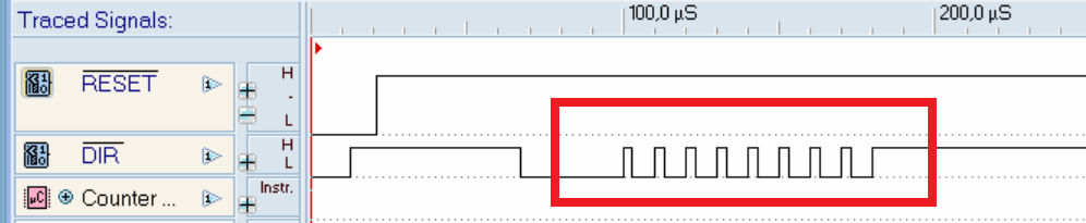
A well-chosen time grid simplifies the placement of repetitive transitions in time, which will be limited to time instants that are multiples of the chosen grid step (500 nS in the screenshot below).
Measuring Times using Time Cursors
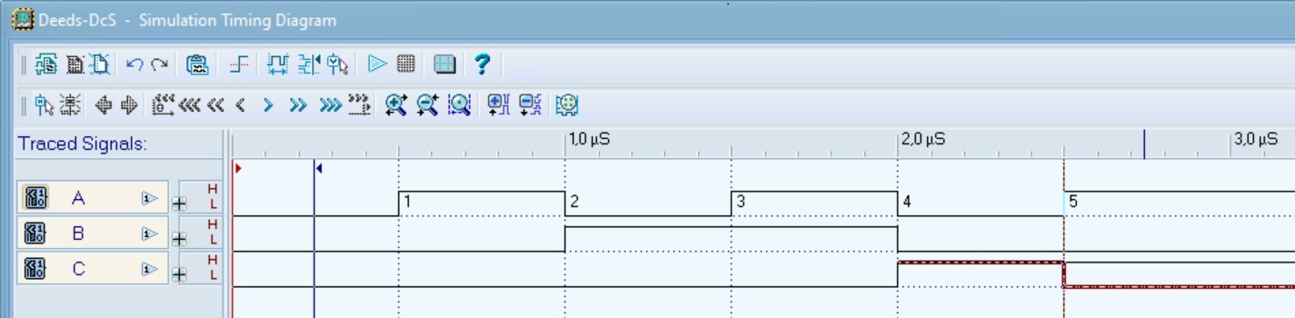
In the example below, the yellow arrow at the top shows the tool bar command that allows you to position the time cursors. The two green arrows indicate the two cursors 'I' and 'II', after having been positioned by the user on the desired edges (the positioning of the two cursors follows a press-drag-release approach).

Time Cursors are 'attracted' to the closest transition under the mouse. If you want to position the cursors freely, however, simply position them a) above a track without transitions, or b) or in the space between two tracks. The orange arrow at the bottom indicates the measurement between the two time cursors.
Magnifier
The 'Magnifier' allows the horizontal time scale to be enlarged in a portion of the diagram, chosen by the user via a pair of vertical cursors. The magnifier is activated by a button on the 'View' toolbar (yellow arrow in the screenshot below).

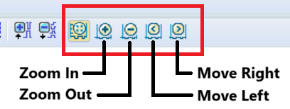
Once activated, the magnified area is colored differently and four buttons appear to the right of the pressed one (highlighted by the red frame). The enlarged area is graphically delimited by two vertical cursors (green and blue arrows).
When the Magnifier is activated, the positioning of the two vertical cursors is automatic. They do not have to be 'placed' by the user, who can however move them as desired. Both cursors are moved with the classic mouse press-drag-release way. The position and magnification can be controlled in several ways, for example via the four buttons on the toolbar, as shown in the figure below.
Alternatively, you can control the position and magnification by clicking the mouse in the different areas. The mouse icon is different from area to area, and turns into a "Little Hand" when it is over the vertical cursors on the sides of the area.
- Left-clicking inside the magnifier area is equivalent to the Zoom In command.
- Right-clicking inside the magnifier area is equivalent to the Zoom Out command.
- Clicking to the left of the magnifier area moves it one step to the left.
- Clicking to the right of the magnifier area moves it one step to the right.
The magnification factor can vary from 'x1' (no magnification) to 'x 8192'.
The magnifier operativity is demonstrated in the following video, which can be downloaded in full resolution here.
Value Cursor
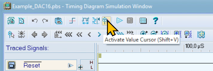
On the top toolbar we find the "Activate value cursor" button.
By clicking on the button we will display the vertical value cursor, attached to the mouse (green arrow in the figure below). A special area of the window also appears, on the right side, organized in the form of a vertical grid. This area will display the list of the values (and the corresponding time transition) of a given track (red ellipse).

By moving the value cursor, the user can choose the desired trace and position in time.
The representation of the data in the value grid area depends on the nature of the chosen trace. For example, in the previous figure we can observe the integer (and binary) values of each sample of the waveform generated by the DAC. The list of values is particularly useful for tracing the sequence of instructions (in Assembly Code) executed by a microprocessor, as shown in the example below.
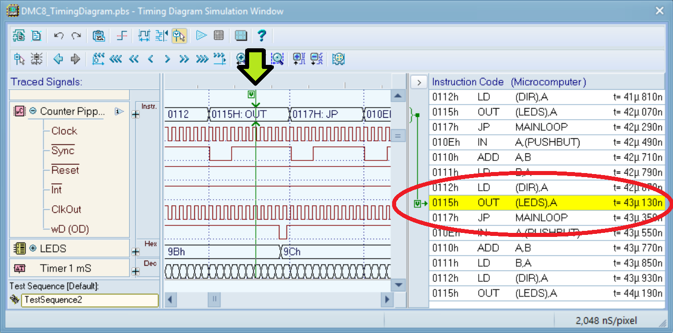
By clicking on a row in the value grid, we automatically activate the Home Cursor and move the Value Cursor and the Diagram View to the time of the selected value.
When you run the simulation, instead, the Value Cursor and the Diagram View automatically move to the time of the last signal transition, selecting the corresponding line in the value grid.
If, after the simulation, you click on the value grid again, both the Home and Value Cursors will be positioned to the time corresponding to the newly selected row. If we restart simulating again the value cursor will reposition to the last transition time, as described above.
To hide the Value Cursor and its grid, we can use the same toolbar button that was used to activate them, or use the close button located on the grid at the top left.
The Value Cursor usage is suggested in the video below, which can be downloaded in full resolution here.
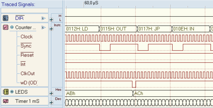
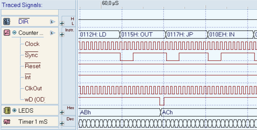
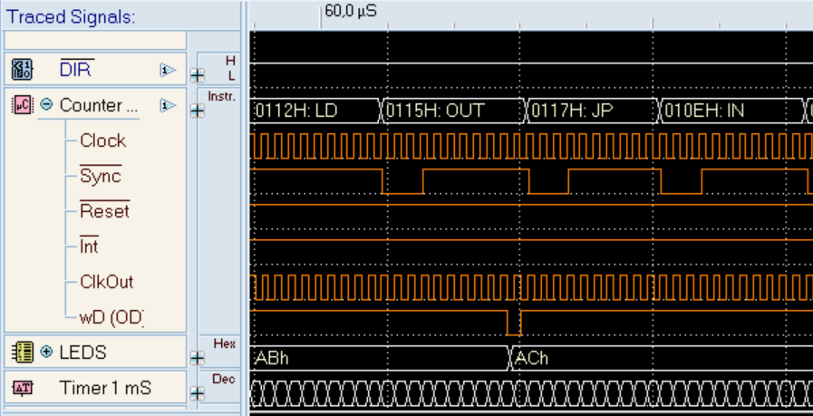
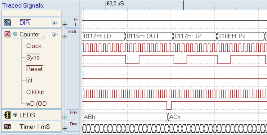
Diagram Color Styles
A button on the command bar allows you to set one of the four available color styles (Cream, Azure, Dark and White).

Azure style is the default (i.e. the old style). The command icon color in the toolbar changes based on the selection made by the user. Below are shown the different color sets, in the menu order.
...To be completed...